Training object detection models for imgproxy

Object detection is a very popular imgproxy Pro feature that allows doing various useful things like performing object-oriented cropping, getting info about objects in images, or censoring detected objects with blurring. The most common use case for object detection is cropping images to focus on human faces; that's why imgproxy's default object detection model is trained to detect faces. However, your use case may require detecting other objects, for example, goods in your online store, cars in your car-sharing app, or animals in your wildlife photo gallery. This guide will show you how to train an AI model compatible with imgproxy to detect objects you need.

TL;DR: If you want to skip the guide and jump straight to the code, you can find the full Jupyter notebook with all the code snippets here.

The object-detection model family of choice for imgproxy is YOLO (You Only Look Once). This family is known for its speed and accuracy, which are crucial for on-the-fly image processing. YOLO models are usually come in different sizes, from tiny models that can run smoothly even on mobile devices to large models that provide the best accuracy but require more computational resources.

Traditionally, object-detection model developers provide models pre-trained on the COCO dataset, which contains 80 classes of objects. If those classes meet your needs, you can just take a pre-trained model and jump straight to the last step of this guide, where we show you how to configure imgproxy to use your model.

At the time this guide is written, the latest YOLO model family member is YOLOv11 from Ultralytics. Ultralytics provides a very handy toolset for training object-detection models, and we will use it in this guide.

Prerequisites

Training an object-detection model requires a lot of computational resources, specifically a powerful GPU. We strongly recommend using a cloud service like Google Colab instead of trying to train the model on your local machine. Google Colab is a Jupyter notebook service that provides free access to computing resources, including GPUs. Since we will use a Jupyter notebook to assemble our training pipeline, Google Colab is a perfect match.

Some experience with Python and Jupyter notebooks would also be handy. However, it's not necessary, as we will provide all the necessary code snippets.

Now, open a new Jupyter notebook, and let's go!

Step 0: Setting a goal

Before you start training your model, you need to decide what objects it should detect. This decision is essential because adding new classes to the model later will require retraining it almost from scratch. It's important to understand that the model can detect only the objects it was trained on.

For the sake of this guide, let's imagine that you're building a pet shop website, so you naturally want imgproxy to focus on our little friends. Let's train a model to detect the following classes of objects: cat, dog, rabbit, hamster, and parrot.

Step 1: Gathering a dataset

Besides choosing the right model, the most important part of training an object-detection model is gathering a good dataset. Object-detection datasets consist of images containing required objects and annotations that describe where those objects are located in the images. The more diverse and representative your dataset is, the better your model will perform. There are several ways to get a dataset:

1. Collecting your own dataset. If this sounds like a lot of work, that's because it is. You need to take or find many suitable photos and annotate them. This is pretty time-consuming, but if your needs are very specific, this may be the only way to get a good dataset. Luckily, there are services that can help you with this task, like Roboflow, Labelbox, or CVAT. We won't cover this method in this guide because it's worth a separate guide on its own.

2. Using an existing dataset. This is the easiest way to get a dataset. Plenty of object-detection datasets are available online. We recommend starting the search from Roboflow Universe or Kaggle Datasets. Roboflow Universe allows you to download datasets in the format you need, dramatically simplifying the process. We won't cover this method in this guide either because it's pretty straightforward.

3. Extracting a subset of an existing dataset. There are many general-purpose object-detection datasets available, like COCO, Open Images, or Objects365. These datasets contain many object classes, but you can extract a subset of the classes you need. We will use this method with the Open Images dataset in this guide.

The Open Images dataset is a large-scale dataset that contains images with annotations for 600 (!) object classes. A good thing about Open Images dataset is that you don't need to download the whole dataset to extract a subset of classes you need: you can use the annotations file to collect IDs of images that contain objects of required classes and download only those images.

Step 1.1: Getting Open Images label names

All the annotations in the Open Images dataset use machine-friendly IDs called LabelName instead of human-readable class names. So, the first thing we need to do is download the boxable class names file and find the LabelName values for the classes we need. Doing this manually is more straightforward than writing a parser.

Now, let's add a code cell to our notebook and put LabelName values for our classes there:

labels = [
  "/m/01yrx",  # Cat
  "/m/0bt9lr", # Dog
  "/m/06mf6",  # Rabbit
  "/m/03qrc",  # Hamster
  "/m/0gv1x",  # Parrot
]

Step 1.2: Downloading images and annotations

Let's create a directory for our dataset first:

import os

dataset_root = "./dataset" # @param {type:"string"}
dataset_root = os.path.abspath(dataset_root)

os.makedirs(dataset_root, exist_ok=True)

The @param {type:"string"} comment tells Jupyter to create an input field for this variable. You can change the default value to set the directory name you like.

Now, let's download the annotations files for training and validation sets. Add the following code cell to your notebook:

!wget "https://storage.googleapis.com/openimages/v6/oidv6-train-annotations-bbox.csv" -O "{dataset_root}/boxes-train.csv"
!wget "https://storage.googleapis.com/openimages/v5/validation-annotations-bbox.csv" -O "{dataset_root}/boxes-val.csv"

Now, we need to filter the annotations to get ones that annotate objects of classes we need and convert them to the YOLO format. In the YOLO dataset format, each image has a corresponding .txt file with the same name containing one line for each object in the image. Each line has the following format:

<class_id> <center_x> <center_y> <width> <height>

<class_id> is the index of the class in the labels list, <center_x> and <center_y> are the coordinates of the object's center, and <width> and <height> is the object's width and height.

We will also need to download the images themselves. We can do this in parallel with filtering annotations to save time, so get ready for a big code snippet! Add the following code cell to your notebook:

!pip install boto3 botocore tqdm

import os
import boto3
import botocore
from tqdm.notebook import tqdm
from concurrent import futures

class dataset:
  def __init__(self, root, name, s3_dir, labels, csv_path):
    self.root = root
    self.name = name

    self.images_dir = os.path.join(root, name, "images")
    self.labels_dir = os.path.join(root, name, "labels")

    os.makedirs(self.images_dir, exist_ok=True)
    os.makedirs(self.labels_dir, exist_ok=True)

    self.s3_dir = s3_dir
    self.s3_bucket = boto3.resource(
      's3',
      config=botocore.config.Config(signature_version=botocore.UNSIGNED, max_pool_connections=35)
    ).Bucket("open-images-dataset")

    self.labels = labels
    self.csv_path = csv_path


  def download_image(self, image_id, boxes):
    path = os.path.join(self.images_dir, f"{image_id}.jpg")

    try:
      self.s3_bucket.download_file(f"{self.s3_dir}/{image_id}.jpg", path)
    except Exception as inst:
      print(f"Downloading error: {inst}")
      return

    labels_path = os.path.join(self.labels_dir, f"{image_id}.txt")

    with open(labels_path, "w") as labels_f:
      for box in boxes:
        cls, x1, y1, x2, y2 = box

        cx = (x1 + x2) / 2
        cy = (y1 + y2) / 2
        w = x2 - x1
        h = y2 - y1

        labels_f.write(f"{cls} {cx} {cy} {w} {h}\n")

      labels_f.close()


  def download_dataset(self, max_images):
    f = open(self.csv_path, "r")

    num_images = 0
    num_cls_images = {}

    image_id = None
    boxes = []
    has_good_boxes = False
    has_bad_boxes = False

    # Skip header
    f.readline()

    pbar = tqdm(total=max_images * len(self.labels), desc=f"Selecting {self.name} images", leave=True)

    executor = futures.ThreadPoolExecutor(max_workers=30)
    all_futures = []

    while True:
      new_image_id = None

      line = f.readline()

      if line != "":
        split = line.strip().split(",")

        new_image_id = split[0]
        label_name = split[2]
        x_min = float(split[4])
        x_max = float(split[5])
        y_min = float(split[6])
        y_max = float(split[7])
        group_of = split[10]
        inside = split[12]

      # The image ID changed, it's time to download the image and reset the state
      if new_image_id != image_id:
        if has_good_boxes and not has_bad_boxes:
          all_futures.append(executor.submit(self.download_image, image_id, boxes))

          pbar.update(len(boxes))

          num_images += 1

          for class_id in set(b[0] for b in boxes):
            num_cls_images[class_id] = num_cls_images.get(class_id, 0) + 1

          had_enough = True
          # Check if we've found enough images for each class
          for class_id in range(len(self.labels)):
            had_enough = had_enough and num_cls_images.get(class_id, 0) >= max_images
          # If we've found enough images, stop
          if had_enough:
            break

        image_id = new_image_id
        boxes = []
        has_good_boxes = False
        has_bad_boxes = False

      if image_id == None:
        break

      if label_name in self.labels:
          if inside == "0" and group_of == "0":
            class_id = self.labels.index(label_name)

            has_good_boxes = has_good_boxes or num_cls_images.get(class_id, 0) < max_images

            boxes.append((class_id, x_min, y_min, x_max, y_max))
          else:
            has_bad_boxes = True

    pbar.close()

    print(f"Selected {self.name} images:")
    for class_id in range(len(self.labels)):
      print(f"{self.labels[class_id]}: {num_cls_images.get(class_id, 0)}")

    pbar = tqdm(total=num_images, desc=f"Downloading {self.name} images", leave=True)

    for future in futures.as_completed(all_futures):
      future.result()
      pbar.update(1)

    pbar.close()

It may look scary, so let's break down what the dataset class does:

• The class's constructor takes the dataset's root directory, the dataset's name (train, val, etc.), the Open Images S3 directory where the images are stored, the list of labels we want to detect, and the path to the annotations CSV file.

• The download_dataset takes the target number of images that should be selected for each class. It reads the annotations CSV file line by line, filters out the annotations for the classes we need, downloads the images, and converts the annotations to the YOLO format.

This helper class organizes the dataset files in a way that is required by the Ultralytics toolset:

<dataset_root>
  train/
    images/
      <image_id>.jpg
    labels/
      <image_id>.txt
  val/
    images/
      <image_id>.jpg
    labels/
      <image_id>.txt

Now when we have the helper class, we can finally download the dataset. Add the following code cell to your notebook:

train_ds = dataset(
  dataset_root,
  "train",
  "train",
  labels,
  os.path.join(dataset_root, "boxes-train.csv"),
)
train_ds.download_dataset(5000)

val_ds = dataset(
  dataset_root,
  "val",
  "validation",
  labels,
  os.path.join(dataset_root, "boxes-val.csv"),
)
val_ds.download_dataset(1000)

Here's what we see in this cell output:

Selected train images:
/m/01yrx: 5012
/m/0bt9lr: 5036
/m/06mf6: 1133
/m/03qrc: 448
/m/0gv1x: 1396

Selected val images:
/m/01yrx: 344
/m/0bt9lr: 1002
/m/06mf6: 64
/m/03qrc: 28
/m/0gv1x: 74

You may notice that we've selected more images than we need for some classes. Though the download_dataset method stops selecting new images for a certain class when it reaches the target number, the other selected images may contain objects of this class as well. This is not a problem, as the model will learn from these images too.

On the other hand, we may not have selected enough images for some classes. This is simply because there are not enough images in the Open Images dataset that contain objects of these classes. We can't do anything about this; the model will have to learn from fewer examples for these classes.

The last thing left to do before we start training is to create a data file that will tell the Ultralytics toolset where to find the images and annotations and what classes the dataset contains. Add the following code cell to your notebook:

%%writefile {dataset_root}/data.yaml

train: ../train/images
val: ../val/images
test:

names:
  - Cat     # /m/01yrx
  - Dog     # /m/0bt9lr
  - Rabbit  # /m/06mf6
  - Hamster # /m/03qrc
  - Parrot  # /m/0gv1x

%%writefile is a Jupyter magic command that writes the cell's content to a file. In this case, we write the content of the cell to the data.yaml file in the dataset root directory.

Step 2: Training the model

At last, we are ready to train our model! Let's install the Ultralytics toolset first:

!pip install ultralytics
import ultralytics
ultralytics.checks()

This code cell will install the Ultralytics toolset and check if everything is operational. If you see no errors, you are good to go!

One more thing that I'd recommend to do before starting the training is to activate TensorBoard to monitor the training process. In Google Colab, you can do this with a simple code cell:

%load_ext tensorboard
%tensorboard --logdir ./OID-pets

Finally, let's start the training! Add the following code cell to your notebook:

!yolo train \
  model=yolo11s.pt \
  data={dataset_root}/data.yaml \
  epochs=300 \
  patience=50 \
  imgsz=640 \
  batch=0.7 \
  cache="disk" \
  project="OID-pets" \
  name="train" \
  exist_ok=True \
  degrees=45 \
  flipud=0.5 \
  fliplr=0.5

Let's break down the parameters we pass to the yolo train command:

• model tells the toolset which model to use. We use the yolo11s.pt model, which is the second smallest model in the YOLOv11 family. We find this model to be a good balance between speed and accuracy.

• data points to the data.yaml file we've created earlier.

• epochs is the number of training epochs. We set it to 300, but you can adjust this value based on the training progress.

• patience is the number of epochs without improvement, after which the training will stop. 300 epochs that we set earlier is quite a large number for our task, so we want to stop early if the model doesn't improve.

• imgsz is the size of the input images; we set it to 640x640 pixels. This is the default value, yet I prefer to set it explicitly.

• batch is the batch size, which defines how many images the model will be trained on in one step. When this value is less than 1, it's interpreted as a fraction of the available GPU memory. We set it to 0.7, which means that the training will choose the batch size that uses 70% of the available GPU memory.

• cache tells the toolset to cache the dataset to improve the training speed. We set it to "disk" to cache the dataset on the disk.

• project is the project's name. The toolset will create a directory with this name in the current working directory to store the training results.

• name is the name of the training run. The toolset will create a directory with this name inside the project directory to store the training results for this run. When you're experimenting with your model, you may want to omit this parameter to make the Ultralytics toolset generate a unique name for you, but for our task, it's okay to set it statically.

• exist_ok tells the toolset not to fail if the project or run directory already exists.

• degrees, flipud, and fliplr are data augmentation parameters. Data augmentation is a technique used to help the model generalize better by applying random transformations to the input images.

After you run this cell, the training process will start. It will eventually start generating output like this:

Epoch    GPU_mem   box_loss   cls_loss   dfl_loss  Instances       Size
1/300      34.6G      1.627       2.64      1.979         55        640: 100% 95/95 [00:59<00:00,  1.60it/s]
           Class     Images  Instances      Box(P          R      mAP50  mAP50-95): 100% 6/6 [00:08<00:00,  1.46s/it]
             all       1508       1782      0.623      0.705      0.693      0.366

The first two lines show the training progress for the current epoch. The last two lines show the model's performance on the validation set. The mAP50 value is the mean average precision, a common metric for object detection models. The higher this value, the better the model performs. You may notice that this value drops in the first few epochs, but this is normal; it will start to grow after some time.

The other metrics are precision (P) and recall (R). You can read more about these metrics in the Ultralytics documentation.

These metrics may be confusing if you have just started diving into the machine-learning world. Don't worry! The vast majority of machine learning toolsets automatically select the best model for you, and the Ultralytics toolset is no exception. If you want to estimate the training progress, you can simply monitor the mAP50 value. Don't worry if it starts to drop at some point; the toolset saves the latest and the best models after each epoch, so you won't lose the best model.

Remember I recommended activating TensorBoard earlier? That's because it shows the training progress more visually: ✨graphs✨! Scroll back to the TensorBoard cell, refresh the TensorBoard interface, and you will see something like this:

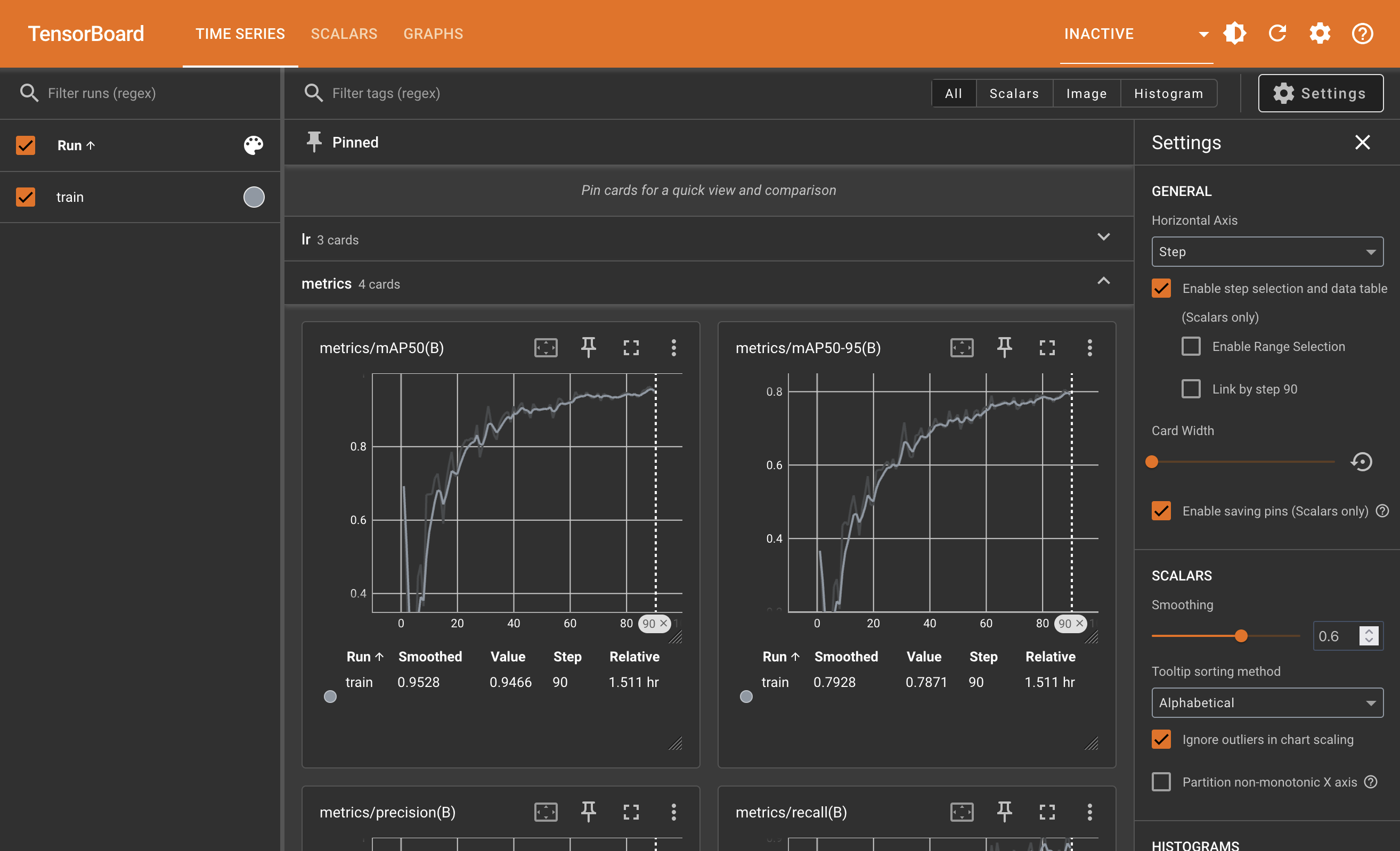
Okay, now you can sit back and relax while the model is training. It may take several hours, even on a powerful GPU, so you may want to do something else in the meantime. When the training is finished, you will see the final metrics in the output, and the best model will be saved in the best.pt file in the run directory.

Step 3: Testing the model

The training process is finished, but we only have a lot of text output and some graphs so far. Not much fun, huh? Show me images!

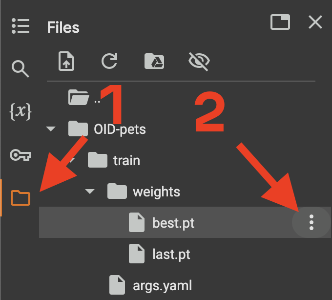
Hold up a bit! Though we are ready to test the model, it's better to download the best model to your local machine first. Google Colab is a temporary environment, and you may lose your data. It's better to be safe than sorry! Open the file browser in the left sidebar, navigate to the OID-pets/train/weights directory, and download the best.pt file:

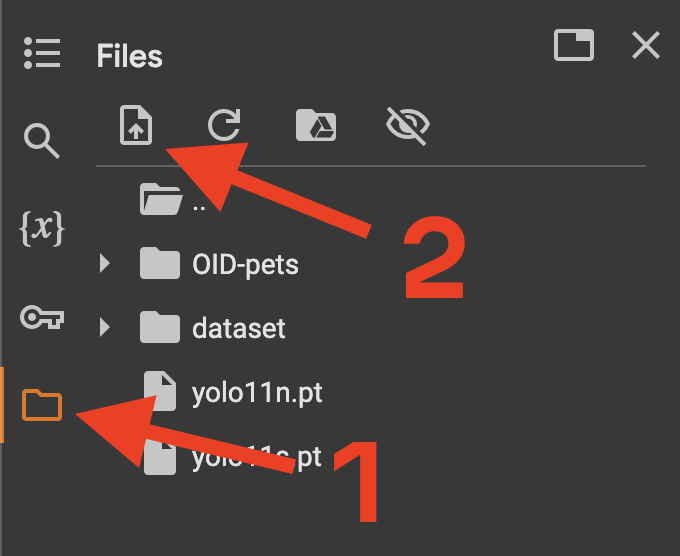
Now, when we secure our training results, let's test the model! First, we need test images. I usually search for test subjects on Unsplash. Download some photos of cute furballs and upload them to your Google Colab session:

The testing process is done with the yolo predict command. Add the following code cell to your notebook:

import os
import matplotlib.pyplot as plt
import matplotlib.image as mpimg

test_image_path = "./test.jpg" # @param {type:"string"}
test_image_name = os.path.basename(os.path.realpath(test_image_path))
result_path = "OID-pets/predict/" + test_image_name

!yolo predict \
  model="OID-pets/train/weights/best.pt" \
  source=$test_image_path \
  imgsz=640 \
  project="OID-pets" \
  name="predict" \
  exist_ok=True

img = mpimg.imread(result_path)
plt.figure(figsize=(8, 8))
plt.imshow(img)
plt.tight_layout()
plt.axis('off')
plt.show()

Change the test_image_path variable to the path of the image you've uploaded.

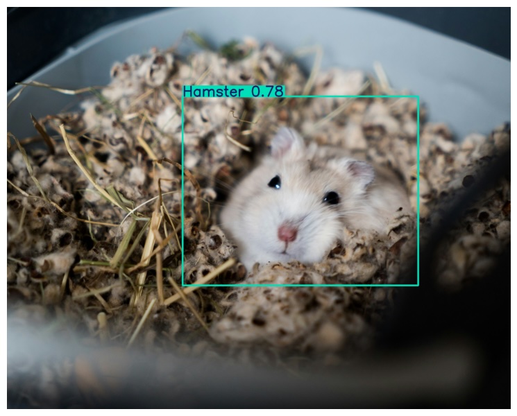
This code cell runs the model on the test image, saves the result to the OID-pets/predict directory, and shows the result in the output. You will see the original image with bounding boxes around the detected objects.

I picked a photo by Björn Antonissen, and here's the result. A hamster is spotted!

Step 4: Configuring imgproxy

Let's do what we've been training the model for: configuring imgproxy to use it!

Step 4.1: Exporting the model to the ONNX format

YOLOv11 models are built with the TensorFlow framework and saved in the .pt format, which imgproxy doesn't support. Instead, imgproxy uses the ONNX format for object detection models. ONNX is a universal neural network format, and the most popular machine-learning frameworks can export models to it. The Ultralytics toolset supports exporting models to the ONNX format with the yolo export command. Add the following code cell to your notebook:

!yolo export \
  model="OID-pets/train/weights/best.pt" \
  format=onnx \
  imgsz=640 \
  simplify=True \
  half=True \
  device=0

!cp OID-pets/train/weights/best.pt ./oid-pets.pt
!cp OID-pets/train/weights/best.onnx ./oid-pets.onnx

This code cell exports the best model to the ONNX format and copies the exported model to the working directory. Let's break down the parameters we pass to the yolo export command:

• model is the path to the model we want to export.

• format tells the toolset which format to export the model to. We set it to onyx.

• imgsz is the size of the input images. We set it to 640x640 pixels, the same as during the training.

• simplify tells the toolset to simplify the model, reducing its size and making it faster.

• half tells the toolset to use half-precision floating-point numbers, which reduces the model's size and speeds it up.

• device specifies which devise the toolset should use when exporting the model. It doesn't affect the model itself. We set it to 0 to use the first GPU.

Now, you can download the oid-pets.onnx file from the file browser in the left sidebar. After you download the file, you can disconnect from the Google Colab session to avoid wasting computation units.

Warning: Google Colab sessions are deleted when disconnected, so ensure you've downloaded all the necessary files before disconnecting.

Step 4.2: Creating a class names file

The next thing we need is a class names file. YOLO models' output doesn't contain class names, only their IDs, so imgproxy needs a file that maps class IDs to class names. Create a file named oid-pets.names with the following content:

cat
dog
rabbit
hamster
parrot

The file contains class names on which the model was trained, one name per line, in the exact order as in the annotations. It's important to understand that this file doesn't affect the model itself; it's only used by imgproxy to map class IDs to class names and vice versa. Adding, removing, or changing class names in this file won't make the model detect another set of classes.

Step 4.3: Building a Docker image

Let's assemble the things we've prepared into a Docker image containing imgproxy configured to use our model. Create a Dockerfile with the following content:

ARG BASE_IMAGE="docker.imgproxy.pro/imgproxy:latest-ml"

FROM ${BASE_IMAGE}

COPY oid-pets.onnx /opt/imgproxy/share/models/oid-pets.onnx
COPY oid-pets.names /opt/imgproxy/share/models/oid-pets.names

ENV IMGPROXY_OBJECT_DETECTION_NET=/opt/imgproxy/share/models/oid-pets.onnx
ENV IMGPROXY_OBJECT_DETECTION_NET_TYPE=yolov11
ENV IMGPROXY_OBJECT_DETECTION_CLASSES=/opt/imgproxy/share/models/oid-pets.names
ENV IMGPROXY_OBJECT_DETECTION_NET_SIZE=640
ENV IMGPROXY_OBJECT_DETECTION_CONFIDENCE_THRESHOLD=0.5

This Dockerfile extends the official imgproxy Pro Docker image and copies the oid-pets.onnx and oid-pets.names files to the image. If you are not an imgproxy Pro user, feel free to request a free trial. Object detection is a Pro feature; the open-source version of imgproxy doesn't support it.

The Dockerfile also sets several environment variables that configure imgproxy to use our model:

• IMGPROXY_OBJECT_DETECTION_NET is the path to the ONNX model file.

• IMGPROXY_OBJECT_DETECTION_NET_TYPE is the model's type. Different YOLO versions have different output formats, so we need to tell imgproxy which output format to expect.

• IMGPROXY_OBJECT_DETECTION_CLASSES is the path to the class names file.

• IMGPROXY_OBJECT_DETECTION_NET_SIZE is the size of the input images. We set it to 640x640 pixels, the same as during the export to ONNX.

• IMGPROXY_OBJECT_DETECTION_CONFIDENCE_THRESHOLD is the confidence threshold. This value tells imgproxy to ignore detections with a confidence score below this threshold. We set it to 0.5, but you can increase the value if you see too many false positives or decrease it if some objects are undetected.

Now, build the Docker image:

docker build -t imgproxy:latest-ml-pets .

You can replace imgproxy:latest-ml-pets with a Docker tag you like.

Step 5: Testing imgproxy with the model

Now, when we have the imgproxy Docker image with our model, let's see it in action! Run the Docker container:

docker run -p 8080:8080 imgproxy:latest-ml-pets

We already have a sample photo of a corgi by Peter Pryharski uploaded to imgproxy's assets server, so let's test the model with it. Let's assume we want to resize the image to fill a 500x500 area and draw bounding boxes around detected objects. Open the following URL in your browser:

http://localhost:8080/unsafe/rs:fill:500:500/g:obj/dd:1/plain/https://assets.imgproxy.net/sample-corgi.jpg

The rs:fill:500:500 option resizes the image to fill a 500x500 area and crops projecting parts. The g:obj option tells imgproxy to use object-oriented gravity during cropping. The dd:1 option tells imgproxy to draw bounding boxes around detected objects.

Here's the result:

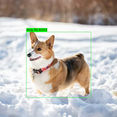
imgproxy detected the dog in the photo and put it in the center of the image! I see this as an absolute win!

Training an object-detection model may look daunting at first glance. But it's just a matter of picking the right dataset and using the right tools. Configuring imgproxy to use your model is even easier: just a few configuration lines. Now that you know the process, you can train models that are compatible with imgproxy for any objects you need. Happy training!

For your convenience, here's the link to the full notebook with all the code snippets.